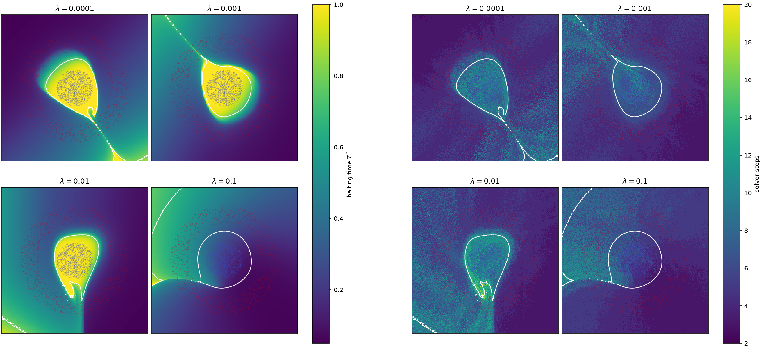
Adaptive Integration Time for Neural ODEs

Two heatmaps showing learned halting time and solver steps for the two-dimensional concentric-annuli task. — Halting-time and solver-step heatmaps for the two-dimensional concentric-annuli task.

Adaptive Integration Time (AIT) allows Neural Ordinary Differential Equations (NODEs) to decide dynamically on how long to integrate for each input. It is posed as a continuous-time analog of Adaptive Computation Time (ACT) (Graves, 2016). AIT-NODEs learn a halting unit that accumulates a halting rate over time, and the solver stops when the accumulated value reaches one. This allows the model to adaptively allocate computation based on the complexity of each input.

The idea¶

A Neural ODE evolves a state $x(t)$ using a learned vector field:

\frac{dx(t)}{dt}=f(x(t),t,\theta) \quad x(0)=x_0.

(1)

And then defines its output as the state at a fixed time $T$ :

x(T)=x(0)+\int_0^T f(x(t),t,\theta)\,dt.

(2)

AIT adds a halting unit $h(x(t),t,\psi)$ . Its output is a positive halting rate, which is accumulated in a scalar state $A(t)$ :

\frac{dA(t)}{dt}=h(x(t),t,\psi), \qquad A(0)=0.

(3)

The solver stops at the first time $T^*$ for which the accumulated value reaches one:

T^*=\inf\{t\geq 0:A(t)=1\}.

(4)

In code, the event function is simply $g(t,z)=1-A(t)$ . This lets an ODE solver locate the stopping point during integration. This can be seen as a continuous time analog of Adaptive Computation Time (Graves, 2016) for Neural ODEs and uses differentiable ODE event handling and event handling per-se (Chen et al., 2021; Shampine and Thompson, 2000).

AIT-NODE¶

The repository’s AITNeuralODE augments the state with the accumulator and a mean-field readout:

z(t)=\begin{bmatrix}x(t)\\A(t)\\\bar{x}(t)\end{bmatrix}, \qquad \frac{dz(t)}{dt}=\begin{bmatrix}f(x(t),t,\theta)\\h(x(t),t,\psi)\\h(x(t),t,\psi)x(t)\end{bmatrix} \qquad z(0)=\begin{bmatrix}x(0)\\0\\0\end{bmatrix}.

(5)

Because $A(t)$ accumulates to one, we can think of our halting unit as a probability density over time. The mean-field readout $\bar{x}(t)$ is the expected state under that density:

\bar{x}(T^*)=\int_0^{T^*} x(t) h(x(t),t,\psi)\,dt=\mathbb{E}_h[x].

(6)

The implementation follows this construction directly:

def _vector_field(self, t, state, args):
    x, A, xbar = state
    hx = jnp.reshape(self.h(t, x, args), ())
    dxbar = hx * x if self.readout is Readout.MEANFIELD else jnp.zeros_like(x)
    return (self.f(t, x, args), hx, dxbar)

The model can also return the endpoint $x(T^*)$ . The repository defaults to the mean-field readout, while the baseline NeuralODE integrates to a fixed $T$ .

Neural ODEs make the connection between depth and integration time explicit (Chen et al., 2019). AIT keeps that continuous-depth view but makes the effective depth depend on the whole state trajectory.

Encouraging less computation¶

AIT adds a ponder penalty to the task loss:

\hat{\mathcal{L}}(X,\Theta)=\mathcal{L}(X,\Theta)+\lambda \mathcal{T}(X,\Theta),

(7)

where $\mathcal{L}(X,\Theta)$ is the task loss and $\mathcal{T}(X,\Theta)$ is the mean halting time for a batch. The training code mirrors the equation:

task = self.task_loss_fn(out, y)
ponder = self.lam * T.mean()
return task + ponder, (task, ponder)

The task loss still determines whether the output is useful. The coefficient $\lambda \geq 0$ controls how strongly training prefers shorter integration.

Because $h$ is monotone, it will eventually reach one, but we can limit the maximum integration time to $T_{max}$ by defining the halting unit as

\tilde{h}(x(t),t,\psi)=h(x(t),t,\psi)+\frac{1}{T_{max}}.

(8)

A positive bias in $h$ also encourages faster halting.

See the code and experiments¶

You can find the code and reproduce the experiments in the AIT-NODE repository.

References¶

Chen, R. T. Q., Rubanova, Y., Bettencourt, J., and Duvenaud, D. (2019). Neural Ordinary Differential Equations. https://arxiv.org/abs/1806.07366
Graves, A. (2017). Adaptive Computation Time for Recurrent Neural Networks. https://arxiv.org/abs/1603.08983
Chen, R. T. Q., Amos, B., and Nickel, M. (2021). Learning Neural Event Functions for Ordinary Differential Equations. https://arxiv.org/abs/2011.03902
Shampine, L. F., and Thompson, S. (2000). “Event location for ordinary differential equations.” Computers & Mathematics with Applications, 39(5), 43-54. https://www.sciencedirect.com/science/article/pii/S0898122100000456

Cite this work¶

If you found this useful, please cite as:

@misc{grassoramos2026ait,
  title  = {Adaptive Integration Time for Neural ODEs},
  author = {Grasso Ramos, Lucas},
  year   = {2026},
  month  = aug,
  url    = {https://github.com/LucasGrasso/AIT}
}